Table of Contents
Introduction
This short project explores machine learning methods for classifying keystrokes based on audio signal. The goal is to determine which key the user is pressing only by analyzing the sound it makes. First, we will look at the data collection method that captures keyboard sounds with precise cuts. Then, we will test different ML algorithms: MFCC features with traditional classifiers, a 1D CNN on raw audio, and neural networks on FFT spectrograms.
Data collection
The keystroke audio collection tool is built with a dual-threaded architecture for precision:
- Audio Thread: Continuously captures microphone input using PortAudio library. The audio is stored in a circular buffer that maintains a rolling window of the last 5 seconds of audio data.
- Keyboard Thread: Monitors key presses in real time using the Windows API. When a key is detected, the system notes the timestamp.
Using the timestamped key press event, a ~400 ms window of audio (100 ms before and 300 ms after the keypress) is extracted from the buffer and saved. Each sample is labeled with the corresponding key.
This architecture ensures that every keystroke is paired with a clean, time-aligned audio snippet.
You can find the full source code for the keystroke audio capture tool here.
A Look at the raw data
| Time Domain | Frequency Domain |
|---|---|
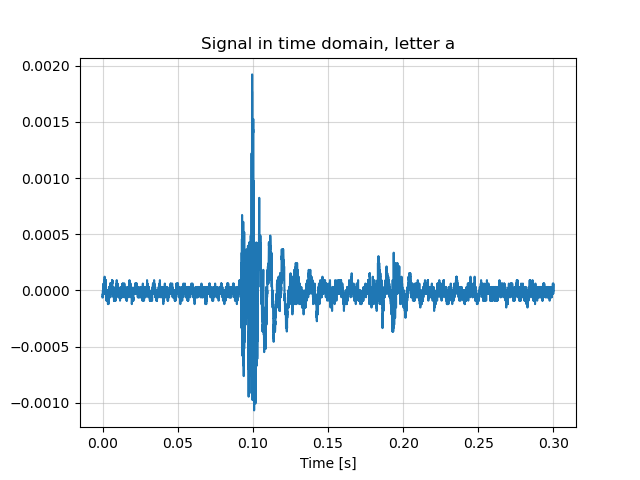 | 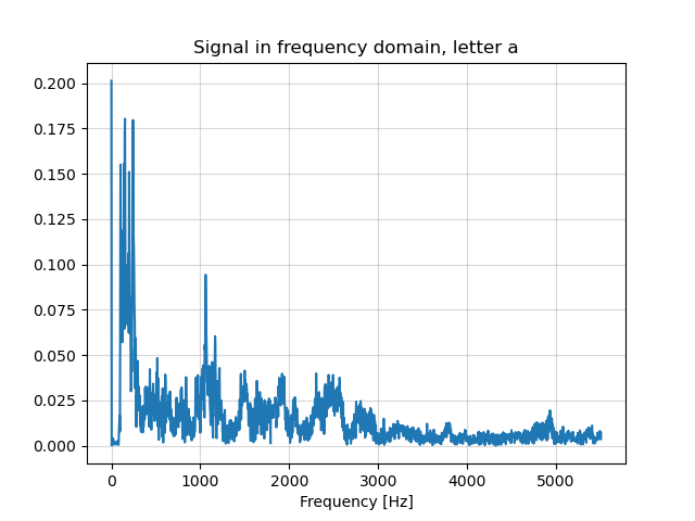 |
In the time domain, the signal shows a sharp initial spike marking the moment of key contact, followed by a secondary smaller peak that likely represents the mechanical rebound.
The frequency domain shows a dominant low-frequency content below 3 kHz, we see a primary peak near DC and a secondary peak around 1 kHz.
MFCC feature extraction with traditional classifiers
The first approach uses Mel-Frequency Cepstral Coefficients (MFCCs) as feature vectors, implementing the mathematical pipeline from scratch:
Signal Windowing: The audio signal is segmented using overlapping Hamming windows of 25 ms duration with a 10 ms hop size.
Spectral Analysis: The windowed signals undergo FFT transformation producing the power spectrum:
$$P(k) = |X(k)|^2$$
where ( X(k) ) is the FFT of the windowed signal.
Mel-Scale Transformation: Linear frequencies are converted to the perceptually-motivated mel-scale using:
$$m = 2595 \times \log_{10}\left(1 + \frac{f}{700}\right)$$
The inverse transformation is:
$$f = 700 \times \left(10^{m/2595} - 1\right)$$
Mel Filterbank: A bank of 26 triangular filters is constructed with mel-spaced center frequencies. Each filter ( H_m(k) ) has the form:
$$ H_m(k) = \begin{cases} 0 & \text{if } k < f(m-1) \newline \frac{k - f(m-1)}{f(m) - f(m-1)} & \text{if } f(m-1) \leq k < f(m) \newline \frac{f(m+1) - k}{f(m+1) - f(m)} & \text{if } f(m) \leq k < f(m+1) \newline 0 & \text{if } k \geq f(m+1) \end{cases} $$
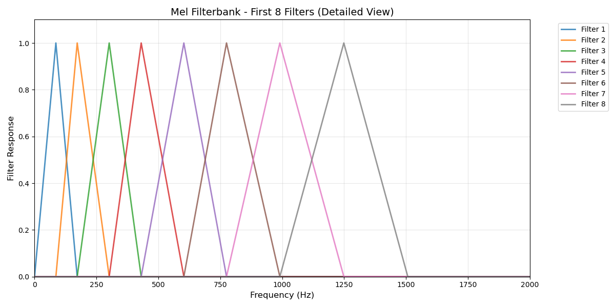
Mel filter banks mimic human hearing by allocating more filters to lower frequencies where we’re more sensitive, and fewer filters to higher frequencies where our discrimination is coarser.
Instead of using all 512+ FFT bins, mel filter banks compress the spectrum into 26 perceptually relevant channels.
Mel Energy Computation:
$$S(m) = \sum_{k=0}^{N/2} P(k) \cdot H_m(k)$$
Logarithmic Compression:
$$\log S(m) = \log(S(m))$$
Discrete Cosine Transform (DCT):
$$C(n) = \sqrt{\frac{2}{M}} \sum_{m=0}^{M-1} \log S(m) \cos\left(\frac{\pi n (m + 0.5)}{M}\right)$$
where $M = 26$ is the number of mel filters and $n = 0, 1, …, 12$ for the first $13$ coefficients.
Feature Aggregation:
$$\bar{C}(n) = \frac{1}{T} \sum_{t=0}^{T-1} C_t(n)$$
These 13-dimensional feature vectors are then fed to traditional classifiers including K-Nearest Neighbors, SVM, Decision Tree, and Random Forest. Evaluation is performed through 5-fold stratified cross-validation with randomized hyperparameter search.
Cross-validation results:
| Model | Train Accuracy | Test Accuracy |
|---|---|---|
| KNN | 1.0000 ± 0.0000 | 0.8084 ± 0.0051 |
| SVM | 0.9510 ± 0.0032 | 0.8588 ± 0.0103 |
| Decision Tree | 0.6098 ± 0.0082 | 0.5255 ± 0.0080 |
| Random Forest | 0.9980 ± 0.0001 | 0.7913 ± 0.0097 |
SVM achieves the best test accuracy (~86%) with reasonable training accuracy, indicating good generalization.
You can find the full source code for this approach here.
One-dimensional convolutional neural network on raw audio
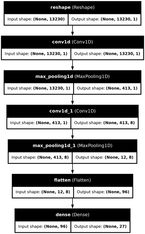
The second approach uses a 1D Convolutional Neural Network (CNN) to learn features directly from the raw audio waveform.

The architecture consists of two convolutional blocks followed by a fully connected classifier. The first convolutional layer uses a single filter with kernel size 128 to capture broad temporal patterns in the 300 ms audio segments, followed by max pooling with stride 32. The second layer applies 8 filters of size 64 to extract more complex hierarchical features, again followed by max pooling. The resulting feature maps are flattened and fed to a dense output layer with 27 neurons (one per key class).
Despite its simplicity, with only 3,268 parameters, this lightweight architecture achieves 95% validation accuracy across all keystroke classes.
You can find the full source code here.
Feedforward neural network on frequency spectrum
In this approach, raw audio signals are transformed into the frequency domain using the Fast Fourier Transform (FFT), converting each 300 ms keystroke sample into a 3,307-dimensional vector representing the spectral magnitude.
These high-dimensional vectors are passed through a fully connected neural network consisting of:
- A dense layer with 32 ReLU-activated neurons,
- A dropout layer (rate 0.5) to reduce overfitting,
- A final output layer with 27 neurons corresponding to each keystroke class.
Despite its shallow structure and modest parameter count (106,747 trainable weights), this model achieves 96.5% validation accuracy.
You can find the full source code here.
Conclusion
This project demonstrates that keystroke classification from audio is a highly feasible task using a variety of machine learning techniques. These results highlight the potential security and privacy implications of acoustic side-channel attacks.