Table of Contents
Introduction
The Nyquist–Shannon theorem is often the first concept introduced in signal processing. It states that if a signal has no frequencies above $f$, then sampling at $2f$ is enough to determine it completely. In other words, to reconstruct a signal without losing information, you must sample at least twice its highest frequency.
In this post, we will look at an intuition behind this theorem by focusing on what happens in the frequency domain.
We will also look at cases where the Nyquist–Shannon criterion can be beaten.
The animations below were made with the library Manim and can be found here.
Aliasing
Aliasing is what happens when we sample too slowly. When the sampling rate falls below the Nyquist rate ($2f$), the sampled points can no longer distinguish the original signal from lower-frequency imposters.
In the animation below, we start with a $3$ Hz signal and gradually reduce the sampling rate. At $5$ Hz below the Nyquist rate of $6$ Hz, the samples now trace out a $2$ Hz wave instead. The original $3$ Hz signal has been “aliased” to a completely different frequency.
From Time-Domain Sampling to Frequency-Domain Replicas
Sampling a continuous signal is mathematically equivalent to multiplying it by a sampling function. This sampling function is a train of Dirac delta functions spaced at intervals of $T_s = \frac{1}{f_s}$: $$s(t) = \sum_{n=-\infty}^{\infty} \delta(t - nT_s)$$ where $f_s$ is the sampling rate.
The fourier transform of the sampling function is: $$ S(f) = \int_{-\infty}^{\infty} \left(\sum_{n=-\infty}^{\infty} \delta(t - nT_s)\right) e^{-i 2\pi f t}\ dt $$ $$ S(f) = \sum_{n=-\infty}^{\infty} \int_{-\infty}^{\infty} \delta(t - nT_s)\ e^{-i 2\pi f t}\ dt $$ Using the shifting property of the dirac: $$ \int_{-\infty}^{\infty} \delta(t - nT_s)\ e^{-i 2\pi f t}\ dt = e^{-i 2\pi f (nT_s)} $$ We have $$ S(f) = \sum_{n=-\infty}^{\infty} e^{-i 2\pi f n T_s} $$ Using the Poisson summation identity: $$ \sum_{n=-\infty}^{\infty} e^{-i 2\pi f n T_s} = \frac{1}{T_s} \sum_{k=-\infty}^{\infty} \delta\left(f - k f_s\right) $$ Therefore: $$ S(f) = \frac{1}{T_s} \sum_{k=-\infty}^{\infty} \delta\left(f - k f_s\right) $$ The result indicates that sampling a signal in the time domain leads to periodic repetitions of its spectrum in the frequency domain, since multiplying in time corresponds to convolution in frequency.
In other words, sampling creates copies of the original spectrum at multiples of $f_s$. When these copies overlap, aliasing occurs. The animation below shows this: as $f_s$ decreases, the replicas move closer until they collide at $f_s < 2 \times bandwidth$.
Compressive sensing
The Nyquist–Shannon theorem sets the fundamental limit for sampling dense, wideband signals, but in certain cases we can go beyond it. If a signal is sparse in some domain (for example, only a few frequencies are active out of many), compressive sensing allows reconstruction from far fewer samples than the Nyquist rate.
We can formulate the compressive sensing problem mathematically as follows.
Let the original signal be $u \in \mathbb{R}^N$. We assume that $u$ can be represented in some basis $B \in \mathbb{R}^{N \times N}$ (such as Fourier or DCT) with sparse coefficients $x \in \mathbb{R}^N$:
$$u = Bx$$
Now, suppose we only observe an undersampled version of the signal through a measurement matrix $M \in \mathbb{R}^{m \times N}$,
which is made up of rows of canonical basis vectors $e_i$ (zeros everywhere and a single one at the sampled position). Here $m \ll N$, so we only keep $m$ samples out of $N$:
$$b = Mu, \quad b \in \mathbb{R}^m$$
Substituting the sparse representation, we obtain:
$$b = MBx$$
Defining $A = MB \in \mathbb{R}^{m \times N}$, we arrive directly at the standard compressive sensing formulation:
$$Ax = b$$
Solving for $x$ will allow us to reconstruct the original signal $u = Bx$ from the samples $b$.
However, this system is underdetermined because $m < N$, meaning there are infinitely many possible solutions.
To recover the true sparse vector $x$, we need an additional criterion.
Instead of minimizing the $L_2$ norm, which spreads energy across all coefficients, we minimize the $L_1$ norm because it promotes sparsity by encouraging most entries of $x$ to be exactly zero.
Ideally, we would minimize the $L_0$ norm, but this problem is NP-hard, so $L_1$ minimization is used because it gives us a convex optimization problem that can scale.
We specifically seek a sparse solution because we know by assumption that $x$ itself is sparse in the chosen basis $B$.
As a reminder, the norms are defined as:
- $L_0$: $|x|_0 = \text{number of nonzero entries in } x$
- $L_1$: $|x|_1 = \sum_i |x_i|$
- $L_2$: $|x|_2 = \sqrt{\sum_i x_i^2}$
To illustrate we can look at a $2D$ example where the equation $a^\top x = b$ represents a straight line: all points $(x_1, x_2)$ that satisfy the linear relation $a_1 x_1 + a_2 x_2 = b$. Geometrically, the set of feasible solutions form a line.
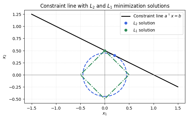
Norm minimization then selects one particular point on this line:
- The $L_2$ solution is the point on the line closest to the origin, i.e. the minimum Euclidean norm solution.
- The $L_1$ solution is the point on the line with the smallest sum of absolute values, which promotes sparsity.
Example: Compressive sensing on a 1D signal
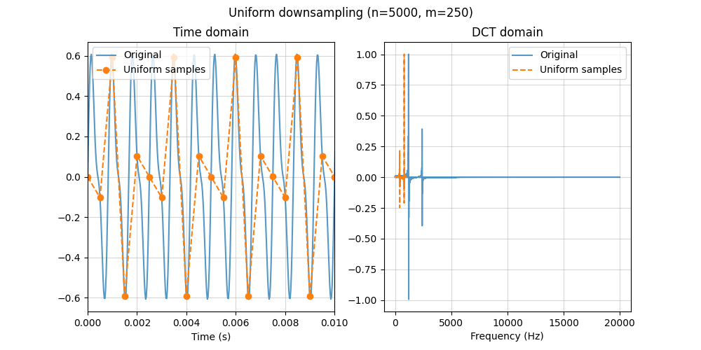
In the first example, we will use a 1D signal that is sparse in the DCT/Fourier domain: a sum of two sinusoids.
You can find the code here
In nature, signals are rarely this sparse, but they are quite sparse nonetheless.
We first undersample the signal on a regular grid (uniform downsampling). As expected from the Nyquist–Shannon rule, once the effective sampling rate drops too low, the sampled points no longer correspond to the original waveform.
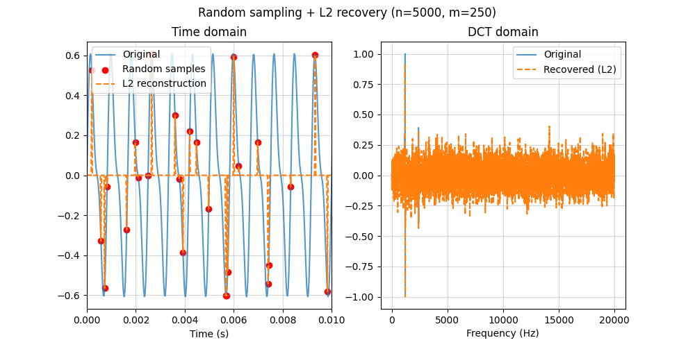
Next, we take the same number of samples at random time locations and reconstruct using an $L_2$ (minimum-norm) solution. This satisfies the measurements, but because $L_2$ does not encourage sparsity, it distributes energy across many frequencies and produces a not so accurate reconstruction.
Finally, we reconstruct from the same random samples using $L_1$ minimization. Here the sparsity condition is explicit: the recovered spectrum concentrates on the true components, and the time-domain signal is reconstructed accurately from the undersampled measurements.
The $L_1$ minimization is solved with CVXPY.
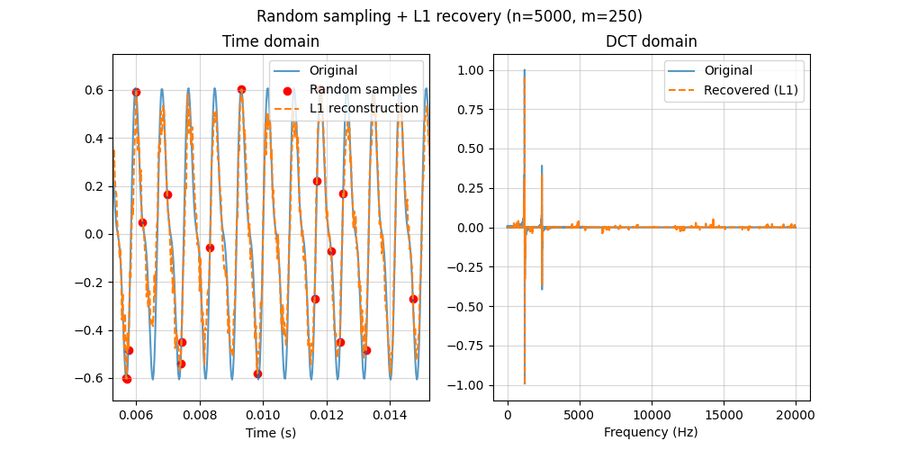
Seeing a full waveform recover from only a few samples can feel almost like magic.
Example: Compressive sensing on a 2D image
Images are a natural domain for compressive sensing, because they tend to be sparse (or at least highly compressible) in a suitable basis.
You can find the code here
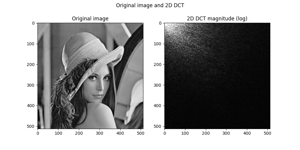
As shown below, the original image and its representation in the 2D DCT domain reveal that most of the energy is concentrated in only a small set of coefficients.
In fact, we can zero out about $98$ % of the DCT coefficients (keeping only the largest $2$ %) and still recover an image that looks very close to the original.
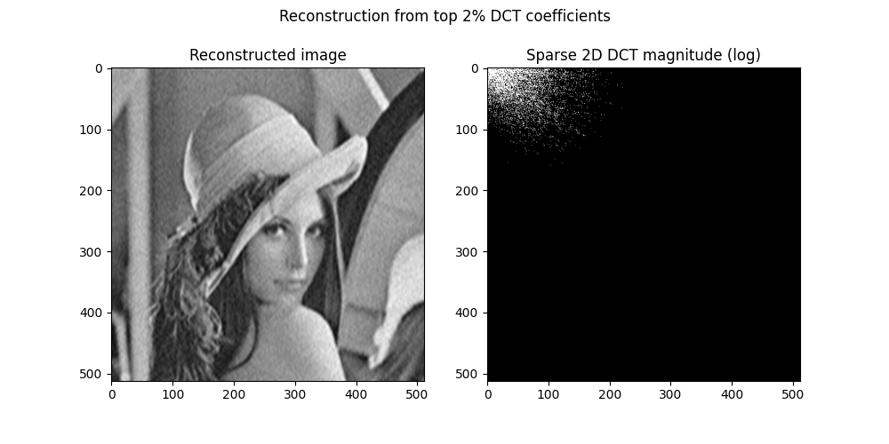
This is exactly the kind of setting where compressive sensing makes sense: if the image is going to be heavily compressed in a sparse domain anyway, why capture every pixel in the first place?
Instead, we can measure only a subset of pixels and let the sparsity prior fill in the rest, recovering the full image from far fewer samples.
We reconstruct using FISTA, a fast gradient-based $L_1$ solver: each iteration takes a gradient step to fit the measured pixels, then applies soft-thresholding to keep the DCT coefficients sparse.
The implementation here uses PyLops. While the same convex problem could be written in CVXPY, for an image of this size it would be far too slow and memory-hungry, so a specialized first-order method like FISTA is the practical choice.
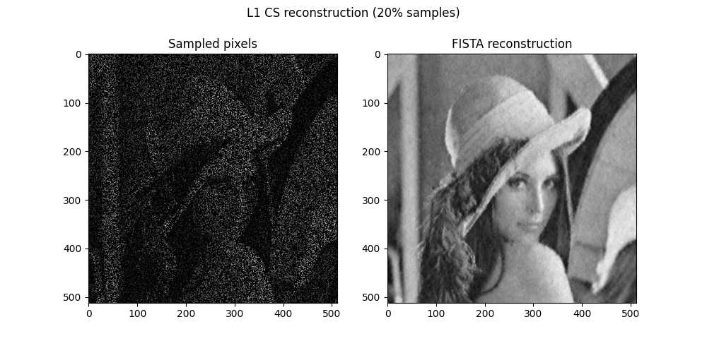
Even with only $20$ % of the pixels measured, the sparse $L_1$ reconstruction recovers most of the image structure remarkably well.
This approach still has clear limitations, though: sparsity in the DCT domain does not mean we can sample at the same extreme rate.
So even if keeping only $2$ % of the DCT coefficients preserves the image, we should not expect equally good reconstructions from only $2$ % of randomly sampled pixels.
Conclusion
Nyquist–Shannon remains the right lens for dense, wideband signals: to avoid aliasing you must sample fast enough to keep spectral replicas separated.
But when a signal is sparse or compressible in a known basis, compressive sensing shows that we can trade samples for computation, recovering the full signal from far fewer measurements by explicitly enforcing sparsity.
The 1D and 2D examples illustrate both the promise and the limits: random sampling plus $L_1$ recovery can beat uniform undersampling, yet the achievable rate depends on how sparse the signal really is and how incoherent the measurements are with the sparsifying basis.
In short, we don’t “break” Nyquist for free — we beat it by adding structure, and paying with optimization.