Table of Contents
Introduction
The Fourier Transform is usually introduced as a way to analyze frequencies in signals. But its importance goes far beyond spectral analysis.
At its core, the Discrete Fourier Transform is a change of basis. It represents a signal using complex exponentials instead of time-domain samples, without altering the underlying information.
Why complex exponentials specifically? And what makes the Fast Fourier Transform fast?
We will answer these questions and conclude with a practical example: recovering a sharp image from motion blur using frequency-domain deconvolution.
The Fourier transform
The Fourier transform correlates the signal with complex exponentials at different frequencies:
$$ X(f) = \int_{-\infty}^{\infty} x(t) e^{-i 2\pi f t} dt $$
For each frequency $f$, we multiply the signal by $e^{-i 2\pi f t}$ and integrate. If that frequency is present, the product accumulates constructively. If not, oscillations cancel out.
$e^{-i 2\pi f t} = \cos(2\pi f t) - i \sin(2\pi f t)$ tests against sine and cosine simultaneously. A pure sine at frequency $f$ correlates zero with a cosine at $f$ (they’re $90°$ out of phase), so we need both components.
The output $X(f)$ is complex: magnitude $|X(f)|$ is the amplitude at frequency $f$, phase $\angle X(f)$ is the timing offset.
The discrete version
When signals are sampled at rate $f_s$, the Discrete Fourier Transform (DFT) replaces the continuous integral with a discrete sum over $N$ samples:
$$ X[k] = \sum_{n=0}^{N-1} x[n] e^{-i 2\pi kn/N} $$
This produces $N$ frequency coefficients at frequencies:
$$ f_k = \frac{k f_s}{N}, \quad k = 0,1,\dots,N-1 $$
The DFT implicitly treats the signal as periodic with period $N$ samples. In other words, the sequence $x[n]$ is assumed to repeat indefinitely in time.
Matrix form and change of basis
The DFT is a matrix multiplication $X = Wx$ where:
$$ W[k, n] = e^{-i 2\pi kn/N} $$
We can view the DFT as a change of basis, expressing the signal in the coordinates of the complex exponential basis.
In fact the columns of the matrix $W$ are orthogonal:
$$ \sum_{n=0}^{N-1} e^{i 2\pi k_1 n/N} \cdot e^{-i 2\pi k_2 n/N} = \sum_{n=0}^{N-1} e^{i 2\pi (k_1-k_2)n/N} $$
When $k_1 = k_2$, every term equals 1, giving $N$. When $k_1 \neq k_2$, this is a geometric series summing to zero (because $e^{i 2\pi(k_1-k_2)} = 1$).
Therefore:
$$ W^* W = NI $$
With this we can infer that the inverse DFT is computed with the matrix $$ W^{-1} = \frac{1}{N} W^* $$
We can also infer the energy preservation, because:
$$ |x|^2 = x^* x = \frac{1}{N} x^* (W^* W) x = \frac{1}{N} (W x)^* (W x) = \frac{1}{N} |X|^2 $$
In other words, representing a signal in the frequency domain preserves its total energy, up to a factor of $1/N$. This result is known as Parseval’s theorem.
Why complex exponentials?
We’ve seen that the DFT projects signals onto a basis of complex exponentials. But why these particular functions? After all, many orthogonal bases exist: wavelets, polynomials, or other function families could mathematically represent signals just as well.
Complex exponentials are special for two reasons: one physical, one algebraic.
Physically, many natural phenomena are inherently oscillatory. Sound waves, electromagnetic radiation, and mechanical vibrations are all naturally described by sinusoids. When we decompose a signal into frequency components, we’re often uncovering the actual physical processes that generated it.
Another reason is algebraic: complex exponentials are the eigenfunctions of Linear Time Invariant (LTI) systems. This property makes them uniquely powerful for analyzing how signals transform through physical systems.
LTI systems and convolution
An LTI system satisfies two properties:
- Linearity: If the system produces output $y_1(t)$ for input $x_1(t)$ and output $y_2(t)$ for input $x_2(t)$, then for any scalars $a$ and $b$, the input $a x_1(t) + b x_2(t)$ produces output $a y_1(t) + b y_2(t)$.
- Time invariance: If the system produces output $y(t)$ for input $x(t)$, then for any delay $\tau$, the input $x(t - \tau)$ produces output $y(t - \tau)$. The system’s behavior does not change over time.
LTI systems appear throughout engineering and science: electrical circuits, acoustic spaces, optical systems, communication channels. Even when a system isn’t perfectly linear or time-invariant, the LTI approximation often provides useful insights.
An LTI system is completely characterized by its impulse response $h(t)$ which is the output when the input is a unit impulse $\delta(t)$. In fact any input can be written as a weighted sum of shifted impulses:
$$ x(t) = \int_{-\infty}^{\infty} x(\tau) \delta(t - \tau) d\tau $$
Using linearity and time invariance, the output becomes:
$$ y(t) = \int_{-\infty}^{\infty} x(\tau) h(t - \tau) d\tau $$
In discrete time with circular boundary conditions, this becomes:
$$ y[m] = \sum_{n=0}^{N-1} x[n] h[(m-n) \bmod N] $$
This circular convolution can be written as matrix multiplication $y = Hx$ where $H$ is a circulant matrix:
$$ H[m, n] = h[(m-n) \bmod N] $$
$$ H = \begin{bmatrix} h[0] & h[N-1] & \cdots & h[1] \newline h[1] & h[0] & \cdots & h[2] \newline \vdots & \vdots & \ddots & \vdots \newline h[N-1] & h[N-2] & \cdots & h[0] \end{bmatrix} $$
Diagonalization by the DFT
The key property is that circulant matrices are diagonalized by the DFT matrix. To see why, we can compute the $(m, k)$ entry of the product $HW$:
$$ \begin{aligned} (HW)[m, k] &= \sum_{n=0}^{N-1} h[(m-n) \bmod N] e^{-i 2\pi nk/N} \end{aligned} $$
Let $r = (m - n) \bmod N$. Then $n \equiv (m - r) \pmod N$. Substituting:
$$ \begin{aligned} (HW)[m, k] &= \sum_{r=0}^{N-1} h[r] e^{-i 2\pi (m-r)k/N} \ &= e^{-i 2\pi mk/N} \underbrace{\sum_{r=0}^{N-1} h[r] e^{i 2\pi rk/N}}_{\lambda_k} \end{aligned} $$
This shows $HW = W\Lambda$, where $$ \Lambda = \text{diag}(\lambda_0, \dots, \lambda_{N-1}). $$
Multiplying by $W^{-1}$ gives:
$$ W^{-1} H W = \Lambda $$
The columns of $W$ are eigenvectors of $H$, and the eigenvalues $\lambda_k$ are simply the complex conjugate DFT of the impulse response.
Geometrically, a matrix multiplication typically rotates and scales a vector in complicated ways. Diagonalization finds a special coordinate system where the transformation only scales along each axis, with no rotation or mixing between dimensions.
For LTI systems, this eigenbasis consists of the complex exponentials. Passing a sinusoid through an LTI system cannot change its frequency; it only scales its amplitude and shifts its phase. The system’s effect on each frequency component is independent and determined by a single complex number $\lambda_k$.
This is why frequency-domain analysis is so powerful: complicated time-domain convolution becomes simple multiplication in the frequency domain.
There is also a computational payoff. Diagonalization transforms the convolution $y = Hx$ from a dense matrix-vector product into element-wise multiplication. In the time domain, computing the convolution directly requires $O(N^2)$ scalar multiplications. Using the DFT’s eigenproperty, we decompose the operation into three steps:
- Transform input to frequency domain
- Multiply by frequency response
- Transform back to time domain
With the Fast Fourier Transform (FFT), steps 1 and 3 each take $O(N \log N)$ operations. The total complexity becomes $O(N \log N)$ instead of $O(N^2)$, a dramatic speedup for large $N$.
The FFT algorithm
The naive DFT requires $O(N^2)$ operations. The Fast Fourier Transform reduces this to $O(N \log N)$ through a divide and conquer strategy.
There isn’t a single FFT algorithm but rather a family of algorithms. The most common is the Cooley-Tukey radix-2 algorithm, which requires $N$ to be a power of 2.
The key insight is that the DFT can be split into even and odd indexed samples. For $N$ a power of 2:
$$ X[k] = \sum_{n=0}^{N-1} x[n] e^{-i 2\pi kn/N} = \sum_{m=0}^{N/2-1} x[2m] e^{-i 2\pi k(2m)/N} + \sum_{m=0}^{N/2-1} x[2m+1] e^{-i 2\pi k(2m+1)/N} $$
Factor out the extra term from the odd sum:
$$ X[k] = \sum_{m=0}^{N/2-1} x[2m] e^{-i 2\pi km/(N/2)} + e^{-i 2\pi k/N} \sum_{m=0}^{N/2-1} x[2m+1] e^{-i 2\pi km/(N/2)} $$
The two sums are DFTs of size $N/2$. Define:
$$ X_{\text{even}}[k] = \sum_{m=0}^{N/2-1} x[2m] e^{-i 2\pi km/(N/2)}, \quad X_{\text{odd}}[k] = \sum_{m=0}^{N/2-1} x[2m+1] e^{-i 2\pi km/(N/2)} $$
Then:
$$ X[k] = X_{\text{even}}[k] + e^{-i 2\pi k/N} X_{\text{odd}}[k] $$
But we need $N$ outputs, not just $N/2$. The half size DFTs are periodic with period $N/2$, so $X_{\text{even}}[k + N/2] = X_{\text{even}}[k]$. For the second half of the output, the twiddle factor picks up a phase shift: $e^{-i 2\pi (k+N/2)/N} = -e^{-i 2\pi k/N}$. This gives:
$$ X[k + N/2] = X_{\text{even}}[k] - e^{-i 2\pi k/N} X_{\text{odd}}[k] $$
Recursively splitting until reaching size 1 (where the DFT is trivial) gives the FFT. The recursion has depth $\log_2 N$, and each level performs $O(N)$ operations, yielding $O(N \log N)$ total complexity.
A practical example: image deconvolution
Deconvolution shows how the DFT’s properties work in practice. The problem: recover a sharp image from a blurred one. This works because blurring is an LTI operation.
You can find the code here
The two-dimensional extension
The 2D DFT extends naturally. For an image $x[m, n]$ of size $M \times N$:
$$ X[k_1, k_2] = \sum_{m=0}^{M-1} \sum_{n=0}^{N-1} x[m, n] e^{-i 2\pi (k_1 m/M + k_2 n/N)} $$
This separates into 1D transforms along each axis.
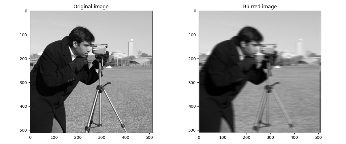
Modeling the blur
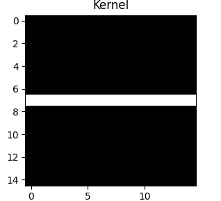
When a camera moves during exposure, each point of light smears across multiple pixels. This is the point spread function, or blur kernel $h$. A stationary, focused camera has a delta function kernel. Motion creates a blur.
We use horizontal motion blur: a 15×15 matrix with ones along the middle row, normalized to sum to 1. This replaces each pixel with the average of its horizontal neighbors.
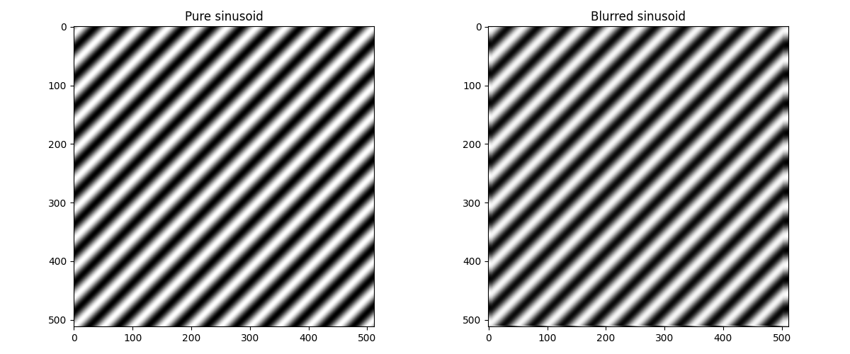
Sinusoid test
When we blur a 2D sinusoid image the output image has the same frequency, The kernel can’t change an eigenfunction’s frequency, only scale and shift it.
Simple deconvolution
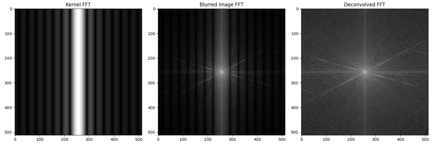
Blurring is $Y[k_1, k_2] = H[k_1, k_2] \cdot X[k_1, k_2]$ in frequency domain. Deconvolution inverts: $X[k_1, k_2] = Y[k_1, k_2] / H[k_1, k_2]$. Add $\epsilon = 10^{-10}$ to avoid division by zero. For noise-free images, this perfectly reconstructs the original image.
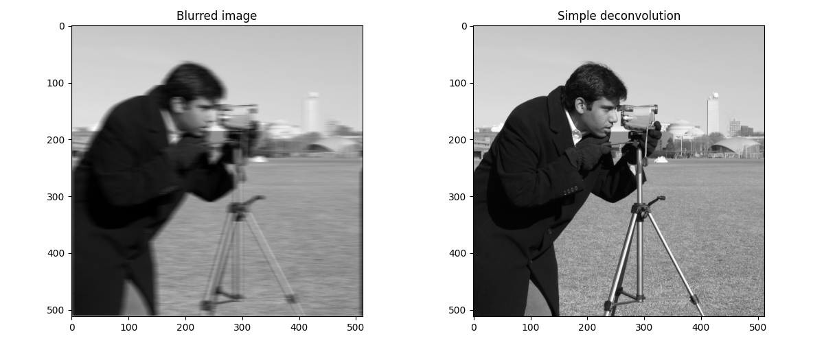
The kernel’s FFT shows which frequencies get attenuated. Horizontal motion blur preserves vertical frequencies but suppresses horizontal frequencies. Deconvolution inverts this: divide by $H$ to restore suppressed frequencies.
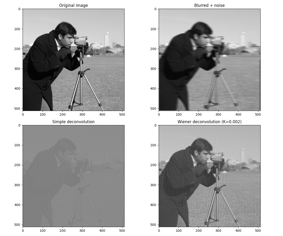
The noise problem
Real images have noise. We will add Gaussian noise with $\sigma = 0.01$ after blurring. Now simple deconvolution fails. Where $|H[k_1, k_2]| \approx 0$, dividing amplifies noise massively. Small noise becomes huge artifacts.
Wiener filtering adds regularization:
$$ W[k_1, k_2] = \frac{H^*[k_1, k_2]}{|H[k_1, k_2]|^2 + K} $$
When $|H|^2 \gg K$: full inversion. When $|H|^2 \ll K$: suppress instead of amplify. The parameter $K$ trades detail for noise. At $K = 0.002$, we recover detail without catastrophic artifacts.
Conclusion
The Discrete Fourier Transform decomposes a signal into frequency components. For an input of $N$ samples, it produces $N$ frequency coefficients. Each coefficient tells you how much of a particular frequency is present in the signal.
The DFT can be understood as a change of basis. The signal is the same, but we’re expressing it in terms of complex exponentials instead of time-domain samples.
The key reason complex exponentials matter is that they’re eigenfunctions of LTI systems. This means convolution in the time domain becomes multiplication in the frequency domain, which is both conceptually simpler and computationally faster with the FFT algorithm.