Simulating fluid

The following article is an implementation and a summarization of this paper:

Real-Time Fluid Dynamics for Games

Link to source code on Github : Simulating fluid source code

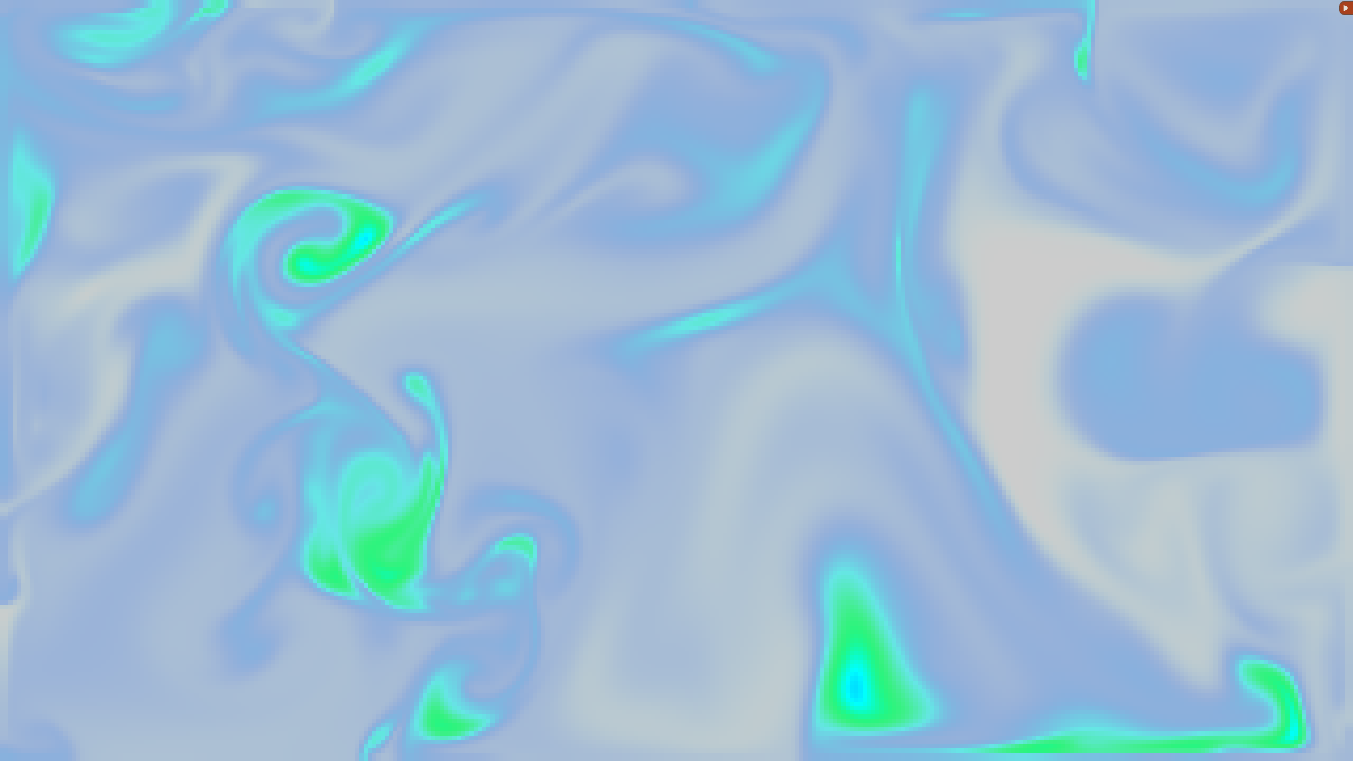
Table of contents

Results

Theoretical background

The Navier-Stokes equations serve as a precise mathematical framework for describing fluid flows found in nature, yet solving them can be quite challenging. Analytical solutions are only feasible in very basic scenarios. In practical applications, the priority is to ensure that simulations are both visually convincing and computationally efficient.

The Navier-Stokes Equations are expressed as follows:

where:

• $\vec{u}$ represents the vector field of the fluid, meaning for each point in space we have a velocity vector.
• $\frac{\partial \vec{u}}{\partial t}$ represents the rate of change of velocity with respect to time. In other words, it describes how the velocity field $\vec{u}$ changes over time at each point in space.
• $- (\vec{u} \cdot \nabla) \vec{u}$ denotes the convective acceleration term. It accounts for how the velocity field “advects” itself, meaning how the velocity field carries and transports fluid particles along its path.

To understand why $- (\vec{u} \cdot \nabla) \vec{u}$ is a vector, consider its expansion: $- (\vec{u} \cdot \nabla) \vec{u} = - \left(u \frac{\partial}{\partial x} + v \frac{\partial}{\partial y} + w \frac{\partial}{\partial z}\right)\vec{u}$ Here, $\vec{u} = (u, v, w)$ represents the velocity field in three dimensions. When we apply the operator $- \left(u \frac{\partial}{\partial x} + v \frac{\partial}{\partial y} + w \frac{\partial}{\partial z}\right)$ to $\vec{u}$ we are essentially taking the derivative of each component of $\vec{u}$ with respect to its corresponding spatial coordinate ($x$, $y$, or $z$) and then multiplying them by the components of $\vec{u}$. Each resulting scalar expression, when taken together, forms a vector. Therefore, $- (\vec{u} \cdot \nabla) \vec{u}$ represents a vector field, as it consists of three scalar components.

• $\nu \nabla ^ 2 \vec{u}$ is the viscous diffusion term. It represents the dissipation of kinetic energy due to viscosity, which tends to smooth out velocity gradients within the fluid.
• $\vec{f}$ represents external forces acting on the fluid.
• $\rho$ is the density field of the fluid, a continuous function which for every point in space tells us the amount of particles present.
• $\frac{\partial \rho}{\partial t}$ represents the rate of change of density with respect to time. It describes how the density of the fluid changes over time at each point in space.
• $-(\vec{u} \cdot \nabla) \rho$ is the convective term for density. It describes how the density field is advected by the velocity field.
• $\kappa \nabla ^ 2 \rho$ is the diffusion term for density. Similar to the viscous diffusion term in the velocity equation, it represents the smoothing out of density gradients within the fluid.
• $s$ represents any source or sink terms contributing to changes in density, such as chemical reactions or heat sources.

Implementation

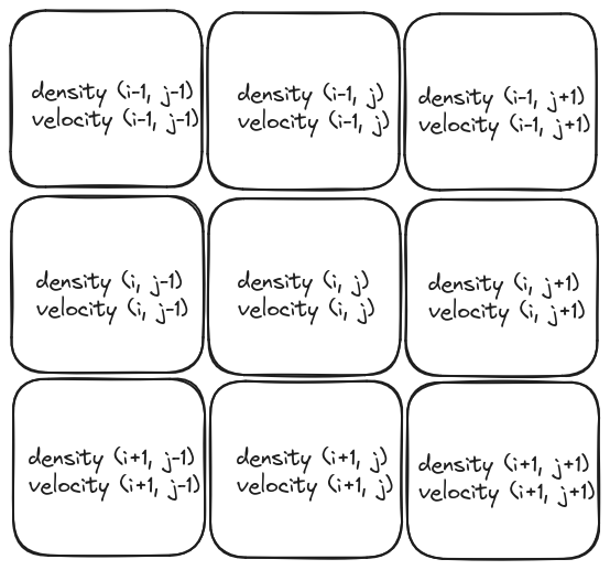
Fluid grid

We will describe the fluid’s behavior by discretizing a 2D plane. This involves dividing the space into a grid of cells and measuring fluid properties (velocity and density) at the center of each cell.

We will define a FluidGrid class as follows:

class FluidGrid {

public:
  int numRows;
  int numColumns;
  std::vector<std::vector<float>> densityGrid;
  std::vector<std::vector<float>> velocityGridX;
  std::vector<std::vector<float>> velocityGridY;
  std::vector<std::vector<float>> densitySourceGrid;
  std::vector<std::vector<float>> velocitySourceGridX;
  std::vector<std::vector<float>> velocitySourceGridY;

private:
  std::vector<std::vector<float>> densityGridOld;
  std::vector<std::vector<float>> velocityGridXOld;
  std::vector<std::vector<float>> velocityGridYOld;

};

densityGrid, velocityGridX, and velocityGridY store the current density and velocity values, while densitySourceGrid, velocitySourceGridX, and velocitySourceGridY indicate the fluid sources, representing the terms $s$ and $\vec{f}$ in the Navier-Stokes equations. Additionally densityGridOld, velocityGridXOld, and velocityGridYOld retain the density and velocity values from the previous calculation.

Solving for density

Initially, we will outline the solution method for a density field in motion within a constant velocity field that remains unchanged over time. Let’s consider the density equation:

Adding source

The first term from the right says that the density increases due to sources, this can be easily implemented with the following function:

void FluidGrid::addSource(int numRows, int numColumns,
                          std::vector<std::vector<float>> &grid,
                          const std::vector<std::vector<float>> &sourceGrid,
                          float timeStep) {
#pragma omp parallel for
  for (int i = 0; i < numRows; ++i) {
    for (int j = 0; j < numColumns; ++j) {
      grid[i][j] += sourceGrid[i][j] * timeStep;
    }
  }
}

#pragma omp parallel for is a component of OpenMP, a library facilitating parallel programming in C/C++. It is employed before a for loop to distribute its iterations among multiple threads. Consequently, the loop iterations can be executed concurrently, thereby diminishing the overall execution time.

Opting to parallelize the outer loop instead of the inner loop is frequently more effective because it minimizes overhead. Each parallel region, initiated by #pragma omp parallel, incurs overhead, such as the creation and destruction of threads.

We can start building out stepDensity method:

void FluidGrid::stepDensity(int diffusionFactor, int gaussSeidelIterations,
                            float timeStep) {
  addSource(numRows, numColumns, densityGrid, densitySourceGrid, timeStep);
}

Diffusion

Diffusion represents the second term in the equation ($\kappa \nabla ^ 2 \rho$), involving the dispersion of density across the grid cells. We will assume that each grid cell can only exchange density with its four immediate neighbors.

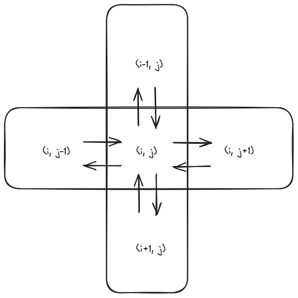
Each cell will lose some of its density to its four neighbors, but will also gain some of the density of each of its neighbors:

Where $a$ is a diffusion factor.

A stable method given by the paper’s author revolves around finding densities which, when diffused backward in time, yields the densities started with, meaning we will solve for $(\rho_{t + \Delta t}[i, j])$ in the equations:

Let’s write the system as a matrix product:

Let $x_t$ and $x_{t +\Delta t}$ be

We have:

where:

Since $(I - aA)$ is very sparse, we can use the simplest iterative solver: Gauss-Seidel relaxation, at iteration $k$:

Therefore we can define out diffusion function as follows:

void FluidGrid::diffuse(int numRows, int numColumns,
                        std::vector<std::vector<float>> &outGrid,
                        const std::vector<std::vector<float>> &inGrid,
                        int gaussSeidelIterations, float factor, int b,
                        float timeStep) {
  float a = timeStep * factor * numRows * numColumns;
  float denominator = 1 + 4 * a;
  for (int k = 0; k < gaussSeidelIterations; ++k) {
#pragma omp parallel for
    for (int i = 0; i < numRows; ++i) {
      for (int j = 0; j < numColumns; ++j) {
        float sum = 0.0f;
        sum += (i > 0) ? inGrid[i - 1][j] : 0.0f;              // Left
        sum += (i < numRows - 1) ? inGrid[i + 1][j] : 0.0f;    // Right
        sum += (j > 0) ? inGrid[i][j - 1] : 0.0f;              // Up
        sum += (j < numColumns - 1) ? inGrid[i][j + 1] : 0.0f; // Down
        outGrid[i][j] = (inGrid[i][j] + a * sum) / (denominator);
      }
    }
    setBounds(numRows, numColumns, outGrid, b);
  }
}

The setBounds function determines how the field behaves at the screen edges. Parameter b specifies which aspect of the field’s boundaries we’re adjusting (density, velocityX, or velocityY):

void FluidGrid::setBounds(int numRows, int numColumns,
                          std::vector<std::vector<float>> &grid, int b) {
#pragma omp parallel for
  for (int i = 1; i < numRows - 1; ++i) {
    grid[i][0] = (b == 2) ? -grid[i][1] : grid[i][1];
    grid[i][numColumns - 1] =
        (b == 2) ? -grid[i][numColumns - 2] : grid[i][numColumns - 2];
  }
#pragma omp parallel for
  for (int j = 1; j < numColumns - 1; ++j) {
    grid[0][j] = (b == 1) ? -grid[1][j] : grid[1][j];
    grid[numRows - 1][j] =
        (b == 1) ? -grid[numRows - 2][j] : grid[numRows - 2][j];
  }
  grid[0][0] = 0.5 * (grid[1][0] + grid[0][1]);
  grid[0][numColumns - 1] =
      0.5 * (grid[1][numColumns - 1] + grid[0][numColumns - 2]);
  grid[numRows - 1][0] = 0.5 * (grid[numRows - 1][1] + grid[numRows - 2][0]);
  grid[numRows - 1][numColumns - 1] = 0.5 * (grid[numRows - 1][numColumns - 2] +
                                             grid[numRows - 2][numColumns - 1]);
}

And we can update the stepDensity method:

void FluidGrid::stepDensity(int diffusionFactor, int gaussSeidelIterations,
                            float timeStep) {
  addSource(numRows, numColumns, densityGrid, densitySourceGrid, timeStep);
  diffuse(numRows, numColumns, densityGridOld, densityGrid,
          gaussSeidelIterations, diffusionFactor, 0, timeStep);
}

Advection

This part makes the density move in the same direction as the velocity (the third term in the equation $-(\vec{u} . \nabla) \rho$).

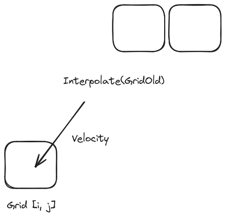
The paper suggests thinking of the density as particles. We look for particles that land exactly in the middle of a grid square in one time step. The density these particles have is figured out by a simple mix of the density where the particles started.

In simpler terms, for each density cell $\rho_{t + \Delta t}[i, j]$ we follow the cell’s center $[i, j]$ backwards through the velocity field. Then $\rho_{t + \Delta t}[i, j]$ will be assigned an interpolated density based on the position where the particles started.

void FluidGrid::advect(int numRows, int numColumns,
                       std::vector<std::vector<float>> &outGrid,
                       const std::vector<std::vector<float>> &inGrid,
                       const std::vector<std::vector<float>> &velocityGridX,
                       const std::vector<std::vector<float>> &velocityGridY,
                       int b, float timeStep) {
  float dtRatio = timeStep * (std::max(numRows, numColumns) - 1);
#pragma omp parallel for
  for (int i = 0; i < numRows; ++i) {
    for (int j = 0; j < numColumns; ++j) {
      float x = i - dtRatio * velocityGridX[i][j];
      float y = j - dtRatio * velocityGridY[i][j];
      x = std::max(0.5f, std::min(static_cast<float>(numRows) - 1.5f, x));
      y = std::max(0.5f, std::min(static_cast<float>(numColumns) - 1.5f, y));
      int x0 = (int)x;
      int y0 = (int)y;
      int x1 = std::min(x0 + 1, (int)numRows - 1);
      int y1 = std::min(y0 + 1, (int)numColumns - 1);
      float sx1 = x - x0;
      float sx0 = 1.0f - sx1;
      float sy1 = y - y0;
      float sy0 = 1.0f - sy1;
      outGrid[i][j] = sx0 * (sy0 * inGrid[x0][y0] + sy1 * inGrid[x0][y1]) +
                      sx1 * (sy0 * inGrid[x1][y0] + sy1 * inGrid[x1][y1]);
    }
  }
  setBounds(numRows, numColumns, outGrid, b);
}

Now we can finalize the stepDensity method:

void FluidGrid::stepDensity(int diffusionFactor, int gaussSeidelIterations,
                            float timeStep) {
  addSource(numRows, numColumns, densityGrid, densitySourceGrid, timeStep);
  diffuse(numRows, numColumns, densityGridOld, densityGrid,
          gaussSeidelIterations, diffusionFactor, 0, timeStep);
  advect(numRows, numColumns, densityGrid, densityGridOld, velocityGridX,
         velocityGridY, 0, timeStep);
  densitySourceGrid = std::vector<std::vector<float>>(
      numRows, std::vector<float>(numColumns, 0.0f));
}

Solving for velocity

Let’s consider the velocity equation:

Adding source

This part is similar to the density equation, therefore we will reuse the same routine addSource

void FluidGrid::stepVelocity(int viscosityFactor, int gaussSeidelIterations,
                             float timeStep) {
  addSource(numRows, numColumns, velocityGridX, velocitySourceGridX, timeStep);
  addSource(numRows, numColumns, velocityGridY, velocitySourceGridY, timeStep);
}

Diffusion

This part is similar to the density equation, therefore we will reuse the same routine diffuse

void FluidGrid::stepVelocity(int viscosityFactor, int gaussSeidelIterations,
                             float timeStep) {
  addSource(numRows, numColumns, velocityGridX, velocitySourceGridX, timeStep);
  addSource(numRows, numColumns, velocityGridY, velocitySourceGridY, timeStep);
  diffuse(numRows, numColumns, velocityGridXOld, velocityGridX,
          gaussSeidelIterations, viscosityFactor, 1, timeStep);
  diffuse(numRows, numColumns, velocityGridYOld, velocityGridY,
          gaussSeidelIterations, viscosityFactor, 2, timeStep);
}

Projection

The Helmholtz decomposition states that any vector field can be resolved into the sum of a curl free vector field and a divergence free vector field, i.e. any vector field $\vec{w}$ can be decomposed into the form:

Where $\nabla \vec{v} = 0$ and $q$ is a scalar field.

The aim is to use projection to make the velocity a mass conserving, in other words to ensure the incompressibility condition of the fluid flow.

Initially, we compute the divergence field of our velocity utilizing the average finite difference method. Following this, we employ a linear solver to solve the Poisson equation. Finally, we subtract the gradient of this field, resulting in a velocity field that conserves mass.

In more details if we have:

Then:

This is a Poisson equation, using the finite difference numerical method to discretize the 2-dimensional Poisson equation:

This equation can be solved iteratively until convergence with Gauss-Seidel relaxation, which gives us the scalar field $q$. We can then subtract the gradient of this field from the original vector field $\vec{w}$ to obtain the divergence-free vector field $\vec{v}$, which conserves mass. This completes the projection step.

void FluidGrid::project(int numRows, int numColumns,
                        std::vector<std::vector<float>> &velocityGridX,
                        std::vector<std::vector<float>> &velocityGridY,
                        std::vector<std::vector<float>> &p,
                        std::vector<std::vector<float>> &div,
                        int gaussSeidelIterations) {
#pragma omp parallel for
  for (int i = 1; i < numRows - 1; ++i) {
    for (int j = 1; j < numColumns - 1; ++j) {
      div[i][j] = -0.5 * (velocityGridX[i + 1][j] - velocityGridX[i - 1][j] +
                          velocityGridY[i][j + 1] - velocityGridY[i][j - 1]);
      p[i][j] = 0.0;
    }
  }
  setBounds(numRows, numColumns, div, 0);
  setBounds(numRows, numColumns, p, 0);
  for (int k = 0; k < gaussSeidelIterations; ++k) {
#pragma omp parallel for
    for (int i = 1; i < numRows - 1; ++i) {
      for (int j = 1; j < numColumns - 1; ++j) {
        p[i][j] = (div[i][j] + p[i - 1][j] + p[i + 1][j] + p[i][j - 1] +
                   p[i][j + 1]) /
                  4;
      }
    }
    setBounds(numRows, numColumns, p, 0);
  }
#pragma omp parallel for
  for (int i = 1; i < numRows - 1; ++i) {
    for (int j = 1; j < numColumns - 1; ++j) {
      velocityGridX[i][j] -= 0.5 * (p[i + 1][j] - p[i - 1][j]);
      velocityGridY[i][j] -= 0.5 * (p[i][j + 1] - p[i][j - 1]);
    }
  }
  setBounds(numRows, numColumns, velocityGridX, 1);
  setBounds(numRows, numColumns, velocityGridY, 2);
}

Advection

This part is similar to the density equation, therefore we will reuse the same routine advect

Now we can finalize the stepVelocity method:

void FluidGrid::stepVelocity(int viscosityFactor, int gaussSeidelIterations,
                             float timeStep) {
  addSource(numRows, numColumns, velocityGridX, velocitySourceGridX, timeStep);
  addSource(numRows, numColumns, velocityGridY, velocitySourceGridY, timeStep);
  diffuse(numRows, numColumns, velocityGridXOld, velocityGridX,
          gaussSeidelIterations, viscosityFactor, 1, timeStep);
  diffuse(numRows, numColumns, velocityGridYOld, velocityGridY,
          gaussSeidelIterations, viscosityFactor, 2, timeStep);
  project(numRows, numColumns, velocityGridXOld, velocityGridYOld,
          velocityGridX, velocityGridY, gaussSeidelIterations);
  advect(numRows, numColumns, velocityGridX, velocityGridXOld, velocityGridXOld,
         velocityGridYOld, 1, timeStep);
  advect(numRows, numColumns, velocityGridY, velocityGridYOld, velocityGridXOld,
         velocityGridYOld, 2, timeStep);
  project(numRows, numColumns, velocityGridX, velocityGridY, velocityGridXOld,
          velocityGridYOld, gaussSeidelIterations);
  velocitySourceGridX = std::vector<std::vector<float>>(
      numRows, std::vector<float>(numColumns, 0.0f));
  velocitySourceGridY = std::vector<std::vector<float>>(
      numRows, std::vector<float>(numColumns, 0.0f));
}

Drawing The Fluid

Naive method

The straight forward method would be to draw each cell in the 2D grid individually using cinder::gl::drawSolidRect, and use the density for the alpha channel.

float cellWidth = (float)getWindowWidth() / numColumns;
float cellHeight = (float)getWindowHeight() / numRows;

for (int i = 0; i < numRows; ++i) {
      for (int j = 0; j < numColumns; ++j) {
        float x = j * cellWidth;
        float y = i * cellHeight;

        float density = densityGrid[i][j];
        ColorA color(1.0f, 1.0f, 1.0f, density);

        gl::color(color);
        gl::drawSolidRect(Rectf(x, y, x + cellWidth, y + cellHeight));
      }
}

However, ths is very slow and inefficient, instead we will use cinder::gl::VboMesh.

VboMesh method

cinder::gl::VboMesh is a class in the Cinder library that serves as a container for a Vertex Buffer Object (VBO). A Vertex Buffer Object (VBO) is a feature in OpenGL that provides methods for uploading vertex data, such as position, normal vector, and color, to the video device for non-immediate-mode rendering1.

We will use HSV (Hue Saturation Value) color coordinate system to have some nice looking cyclic colors:

ci::gl::VboMeshRef fluidMesh;

void FluidApp::initMesh() {
  std::vector<ci::vec2> positions;
  std::vector<ci::ColorA> colors;
  for (int i = 0; i < numRows; ++i) {
    for (int j = 0; j < numColumns; ++j) {
      float x0 = j * gridResolution;
      float y0 = i * gridResolution;
      float x1 = (j + 1) * gridResolution;
      float y1 = (i + 1) * gridResolution;

      positions.push_back(ci::vec2(x0, y0));
      positions.push_back(ci::vec2(x1, y0));
      positions.push_back(ci::vec2(x0, y1));

      positions.push_back(ci::vec2(x1, y0));
      positions.push_back(ci::vec2(x1, y1));
      positions.push_back(ci::vec2(x0, y1));

      for (int k = 0; k < 6; ++k) {
        colors.push_back(
            ci::ColorA(1.0f, 1.0f, 1.0f, fluidGrid.densityGrid[i][j]));
      }
    }
  }

  fluidMesh = ci::gl::VboMesh::create(positions.size(), GL_TRIANGLES,
                                      {ci::gl::VboMesh::Layout()
                                           .attrib(ci::geom::POSITION, 2)
                                           .attrib(ci::geom::COLOR, 4)});
  fluidMesh->bufferAttrib(ci::geom::POSITION, positions);
  fluidMesh->bufferAttrib(ci::geom::COLOR, colors);
}

void FluidApp::updateMesh() {
  std::vector<ci::ColorA> colors;
  for (int i = 0; i < numRows; ++i) {
    for (int j = 0; j < numColumns; ++j) {
      float density = fluidGrid.densityGrid[i][j];
      float hue = 0.5f + 0.1f * sin(2.0f * M_PI * density);
      ci::ColorA color = ci::ColorA(ci::CM_HSV, hue, 1.0f, 1.0f, density);
      for (int k = 0; k < 6; ++k) {
        colors.push_back(color);
      }
    }
  }
  fluidMesh->bufferAttrib(ci::geom::COLOR, colors);
}

Getting user input

In order to make our application interactive, we will utilize the user’s mouse movements as a means to determine density and velocity. The concept is to initiate a click and perform a dragging motion to introduce fluid, with the velocity corresponding to the direction of the drag.

To do so we will use the cinder::app::MouseEvent:

void FluidApp::setup() {
  getWindow()->getSignalMouseDown().connect(
      [this](ci::app::MouseEvent event) { onMouseDown(event); });
  getWindow()->getSignalMouseDrag().connect(
      [this](ci::app::MouseEvent event) { onMouseDrag(event); });
  getWindow()->getSignalMouseUp().connect(
      [this](ci::app::MouseEvent event) { onMouseUp(event); });
}

void FluidApp::onMouseDown(ci::app::MouseEvent event) {
  lastMousePositon = event.getPos();
}

void FluidApp::onMouseDrag(ci::app::MouseEvent event) {
  ci::vec2 currentMousePosition = event.getPos();
  ci::vec2 dragDirection = currentMousePosition - lastMousePositon;

  int i = currentMousePosition.y / gridResolution;
  int j = currentMousePosition.x / gridResolution;

  if (i >= 0 && i < numRows && j >= 0 && j < numColumns) {
    fluidGrid.densitySourceGrid[i][j] += SOURCE_VALUE;
    fluidGrid.velocitySourceGridX[i][j] += dragDirection.x;
    fluidGrid.velocitySourceGridY[i][j] += dragDirection.y;
  }
}

void FluidApp::onMouseUp(ci::app::MouseEvent event) {
  lastMousePositon = ci::vec2(0, 0);
}

That’s all folks, thanks for reading.