Building an Autograd Library from Scratch in C for Simple Neural Networks |

Open Table of contents

Introduction
Neural Networks: A Brief Overview
Derivative Calculation: Symbolic, Numerical and Automatic Differentiation
Implementation
Tests
Examples
- MNSIT
- Paint
Conclusion

Introduction

Autograd is a fundamental component in machine learning frameworks, enabling the automatic computation of gradients for training neural networks. This article will walk you through my journey of writing an Autograd library from scratch (no third-party libraries) in pure C.

The source code is hosted in this repository

Neural Networks: A Brief Overview

At its core, a neural network consists of neurons organized in layers. Each neuron receives input from the previous layer, processes it using a weighted sum, applies an activation function, and passes the output to the next layer.

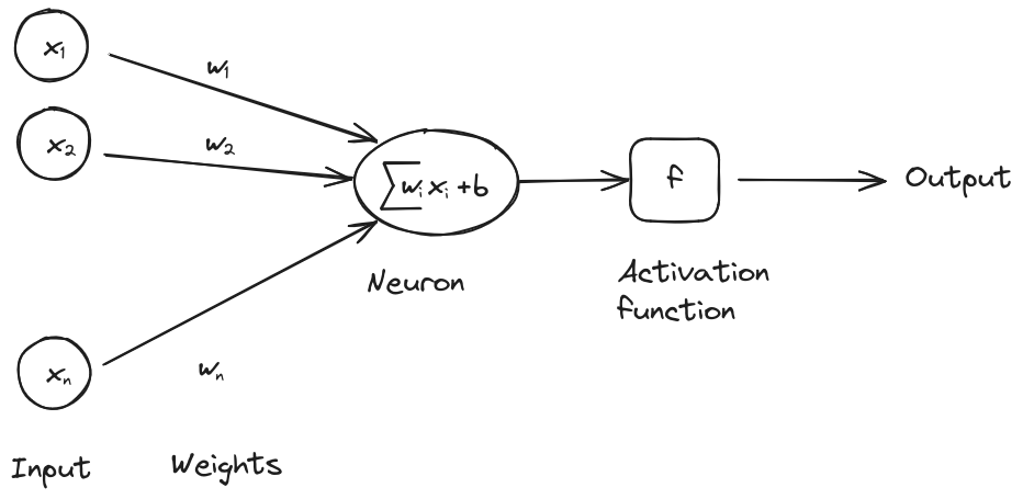
Mathematically, we can express the output of a single neuron as:

y = f(\sum_{i=1}^{n} w_i x_i + b)

where $x_i$ are the inputs, $w_i$ are the weights, $b$ is the bias, and $f$ is the activation function.

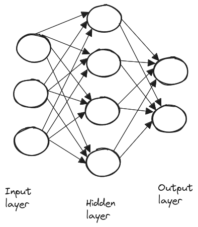
A layer is simply a collection of neurons, and neural networks typically consist of three types of layers: input, hidden, and output layers.

Neural networks learn by adjusting the weights $w_i$ and bias $b$ of each neuron to minimize the error in their predictions. This is done via gradient descent, where the network computes the gradient of the error for each weight and bias and then updates them in the direction that reduces the error.

Derivative Calculation: Symbolic, Numerical and Automatic Differentiation

There are three fundamental ways to calculate derivatives:

Symbolic differentiation: It involves finding the exact derivative of a function using algebraic rules. If the function has a known mathematical expression, we can compute its derivative symbolically. For example for $f(x) = x^2$ the derivative is $f'(x) = 2x$ . This method can lead to unwieldy expressions, especially for functions involving products, quotients, or compositions of multiple functions.
Numerical differentiation: These methods estimate the derivative by using values of the function at specific points. A common finite difference formula for the first derivative is given by $f'(x) = \frac{f(x+h) - f(x)}{h}$ , $h$ is a small step size. However, finite difference methods are not well-suited for neural networks, mainly for efficiency reasons: neural networks typically involve a large number of parameters (weights and biases). Calculating the gradient for each parameter using finite differences would require evaluating the function multiple times, leading to a significant computational overhead.
Automatic differentiation: Automatic differentiation works by breaking down a function into basic mathematical components and creating a graph. In this graph, the nodes represent variables and operations, while the edges connect each operation to its input variables.

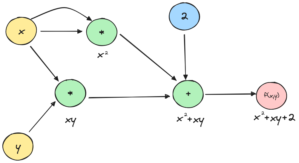
Let’s review a straightforward example of automatic differentiation to make things clearer. Let $f$ be the function $f(x, y) = x^2 +xy +2$ , we will try to find the partial derivatives of $f$ with automatic differentiation.

First let’s represent the function $f$ as a graph:

Now that we have broken the function $f$ to the two mathematical operations $*$ and $+$ which we know how to differentiate, let’s add the local derivatives to the graph.

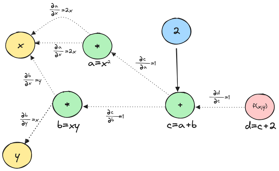
To find the partial derivatives of $f$ we need to find the path from $d$ to $x$ and apply the chain rule. This involves computing the partial derivatives of intermediate variables along this path:

\frac{\partial d}{\partial x} = \frac{\partial d}{\partial c} . \frac{\partial c}{\partial x} = \frac{\partial d}{\partial c} . (\frac{\partial c}{\partial a} . \frac{\partial a}{\partial x} + \frac{\partial c}{\partial b} . \frac{\partial b}{\partial x})

Therefore

\frac{\partial d}{\partial x} = 2x + y

And

\frac{\partial d}{\partial y} = \frac{\partial d}{\partial c} . \frac{\partial c}{\partial y} = \frac{\partial d}{\partial c} . (\frac{\partial c}{\partial a} . \frac{\partial a}{\partial y} + \frac{\partial c}{\partial b} . \frac{\partial b}{\partial y})

Therefore

\frac{\partial d}{\partial y} = x

Using the graph above, we can easily find the answers by tracing paths from $d$ to $x$ or $y$ . Multiply the weights along each path and then sum the results from the different paths.

Therefore, the interest of automatic differentiation is in its ability to efficiently compute gradients for complex functions. It automates the application of the chain rule, ensuring accurate and fast derivatives.

Implementation

N-dimensional array

Before we can implement the Autograd library, we need to create an N-dimensional array (ndarray) library.

The C structure for n-dimensional arrays will include the array’s dimension, total size, shape (size of each dimension), and a pointer to the data. The data type is configurable via a macro.

#define NDARRAY_TYPE double

typedef struct ndarray {
  int dim;
  int size;
  int *shape;
  NDARRAY_TYPE *data;
} ndarray;

Internally, we are representing n-dimensional arrays by a 1D array since it simplifies memory management and access. We can access elements in an n-dimensional array using the shape array. This approach allows us to avoid the need for complex nested loops and makes operations like slicing and reshaping straightforward and performant.

We need functions that operate on the ndarrays, we can distinguish between 3 types of operations:

Unary operations: operations that work on a single ndarray, transforming its elements via element-wise mathematical functions:

ndarray *unary_op_ndarray(ndarray *arr, NDARRAY_TYPE (*op)(NDARRAY_TYPE)) {
  ndarray *n_arr = (ndarray *)malloc(sizeof(ndarray));
  n_arr->dim = arr->dim;
  n_arr->size = arr->size;
  n_arr->shape = (int *)malloc(arr->dim * sizeof(int));
  for (int i = 0; i < arr->dim; i++) {
    n_arr->shape[i] = arr->shape[i];
  }
  n_arr->data = (NDARRAY_TYPE *)malloc(arr->size * sizeof(NDARRAY_TYPE));
  for (int i = 0; i < arr->size; i++) {
    n_arr->data[i] = op(arr->data[i]);
  }

  return n_arr;
}

Binary operations: operations that combine two ndarrays element-wise. These include arithmetic operations (addition, subtraction, multiplication, division). We will also support broadcasting, which allows operations on ndarrays of different but compatible shapes, making it possible to add a vector to a matrix for example which adds the vector to each row of the matrix.

ndarray *binary_op_ndarray(ndarray *arr1, ndarray *arr2,
                           NDARRAY_TYPE (*op)(NDARRAY_TYPE, NDARRAY_TYPE)) {
  if (arr1->dim != arr2->dim) {
    printf("Incompatible dimensions");
    return NULL;
  }
  for (int i = 0; i < arr1->dim; i++) {
    if ((arr1->shape[i] != arr2->shape[i]) &&
        (arr1->shape[i] != 1 && arr2->shape[i] != 1)) {
      printf("Incompatible dimensions");
      return NULL;
    }
  }
  int dim = arr1->dim;
  int *shape = (int *)malloc(dim * sizeof(int));
  for (int i = 0; i < dim; i++) {
    int shape1 = arr1->shape[i];
    int shape2 = arr2->shape[i];
    shape[i] = shape1 > shape2 ? shape1 : shape2;
  }
  ndarray *arr = zeros_ndarray(dim, shape);
  free(shape);
  for (int i = 0; i < arr->size; i++) {
    int idx1 = 0, idx2 = 0, temp = i, stride1 = 1, stride2 = 1;
    for (int j = arr->dim - 1; j >= 0; j--) {
      int shape1 = arr1->shape[j];
      int shape2 = arr2->shape[j];
      idx1 += (temp % shape1) * stride1;
      idx2 += (temp % shape2) * stride2;
      stride1 *= shape1;
      stride2 *= shape2;
      temp /= (shape1 > shape2 ? shape1 : shape2);
    }
    arr->data[i] =
        op(arr1->data[idx1 % arr1->size], arr2->data[idx2 % arr2->size]);
  }
  return arr;
}

Reduce operations: operations that collapse one or more dimensions of an ndarray, producing a result with fewer dimensions. Examples include sum, mean, max, and min along specified axes.

static int get_offset(ndarray *arr, const int *position, int pdim) {
  unsigned int offset = 0;
  unsigned int len = arr->size;
  for (int i = 0; i < pdim; i++) {
    len /= arr->shape[i];
    offset += position[i] * len;
  }
  return offset;
}

void reduce_ndarray_helper(ndarray *arr, ndarray *n_arr, int *position,
                           NDARRAY_TYPE (*op)(NDARRAY_TYPE, NDARRAY_TYPE),
                           int axis, int dim) {
  if (dim >= arr->dim) {
    int rdim = n_arr->dim;
    int n_position[rdim];
    for (int i = 0; i < rdim; i++) {
      n_position[i] = (i == axis) ? 0 : position[i];
    }
    int offset_arr = get_offset(arr, position, arr->dim);
    int offset_narr = get_offset(n_arr, n_position, n_arr->dim);
    n_arr->data[offset_narr] =
        (dim == axis) ? arr->data[offset_arr]
                      : op(n_arr->data[offset_narr], arr->data[offset_arr]);

    return;
  }
  for (int i = 0; i < arr->shape[dim]; i++) {
    position[dim] = i;
    reduce_ndarray_helper(arr, n_arr, position, op, axis, dim + 1);
  }
}

ndarray *reduce_ndarray(ndarray *arr,
                        NDARRAY_TYPE (*op)(NDARRAY_TYPE, NDARRAY_TYPE),
                        int axis, NDARRAY_TYPE initial_value) {
  int *shape = (int *)malloc(arr->dim * sizeof(int));
  for (int i = 0; i < arr->dim; i++) {
    shape[i] = (i == axis) ? 1 : arr->shape[i];
  }
  ndarray *n_arr = full_ndarray(arr->dim, shape, initial_value);
  free(shape);
  int position[arr->dim];
  reduce_ndarray_helper(arr, n_arr, position, op, axis, 0);

  return n_arr;
}

For more info check ndarray.c

Variable node

Let us now implement the structure that will make it possible to use Autograd. We will define a representation of a node in the autograd graph:

typedef struct variable {
  ndarray *val;
  ndarray *grad;
  struct variable **children;
  int n_children;
  void (*backward)(struct variable *);
  int ref_count;
} variable;

ndarray *val : This pointer holds the actual value of the variable stored as a ndarray.
ndarray *grad : This pointer stores the gradient of the variable, which is essential for backpropagation.
struct variable **children : A pointer to an array of pointers to other variables. These represent the variables that depend on this one in the computational graph.
int n_children : The number of child variables, used to keep track of the size of the children array.
void (*backward)(struct variable *) : A function pointer to the backward operation for this variable. This function will be called during backpropagation to compute gradients.
int ref_count : A reference counter for memory management, useful for determining when the variable can be safely deallocated.

we will also define operations on variables :

variable *add_variable(variable *var1, variable *var2);
variable *subtract_variable(variable *var1, variable *var2);
variable *multiply_variable(variable *var1, variable *var2);
variable *divide_variable(variable *var1, variable *var2);
variable *power_variable(variable *var1, variable *var2);
variable *negate_variable(variable *var);
variable *exp_variable(variable *var);
variable *log_variable(variable *var);
variable *sum_variable(variable *var, int axis);
variable *relu_variable(variable *var);
variable *sigmoid_variable(variable *var);
variable *softmax_variable(variable *var, int axis);
variable *tanh_variable(variable *var);
variable *matmul_variable(variable *var1, variable *var2);

The idea is to use these building blocks to build what ever function we want, and then when we would want to compute the gradient of set function we would simple call on the backward function:


void build_topology(variable *var, variable ***topology, int *topology_size,
                    variable ***visited, int *visited_size) {
  for (int i = 0; i < *visited_size; ++i) {
    if ((*visited)[i] == var) {
      return;
    }
  }
  *visited =
      (variable **)realloc(*visited, (*visited_size + 1) * sizeof(variable *));
  (*visited)[*visited_size] = var;
  (*visited_size)++;

  for (int i = 0; i < var->n_children; ++i) {
    build_topology(var->children[i], topology, topology_size, visited,
                   visited_size);
  }
  *topology = (variable **)realloc(*topology,
                                   (*topology_size + 1) * sizeof(variable *));
  (*topology)[*topology_size] = var;
  (*topology_size)++;
}

void backward_variable(variable *root_var) {
  variable **topology = NULL;
  int topology_size = 0;
  variable **visited = NULL;
  int visited_size = 0;
  build_topology(root_var, &topology, &topology_size, &visited, &visited_size);
  for (int i = topology_size - 1; i >= 0; --i) {
    if (topology[i]->backward) {
      topology[i]->backward(topology[i]);
    }
  }
  free(topology);
  free(visited);
}

In other words, we implement a topological sorting algorithm to ensure that gradients are computed in the correct order, from the output back to the inputs. This allows for automatic differentiation of complex, nested functions by applying the chain rule systematically through the computational graph.

Let’s took a deeper look into log_variable as an example:

variable *log_variable(variable *var) {
  variable *n_var = (variable *)malloc(sizeof(variable));
  n_var->val = unary_op_ndarray(var->val, log);
  n_var->grad = zeros_ndarray(n_var->val->dim, n_var->val->shape);
  n_var->children = (variable **)malloc(sizeof(variable *));
  n_var->children[0] = var;
  n_var->n_children = 1;
  n_var->backward = log_backward;
  n_var->ref_count = 0;
  var->ref_count++;

  return n_var;
}

The log_variable creates a new variable node that represents the natural logarithm of an input variable. It allocates memory for this new node, computes its value using the logarithm function, initializes its gradient to zero, and sets up the computational graph structure by linking it to its input (child) variable. The function also assigns the appropriate backward function for gradient computation during backpropagation.

If we look at log_backward:

void log_backward(variable *var) {
  ndarray *place_holder;
  ndarray *temp0;
  ndarray *temp1;

  place_holder = var->children[0]->grad;
  temp0 = divide_scalar_ndarray(var->children[0]->val, 1.0);
  temp1 = multiply_ndarray_ndarray(var->grad, temp0);
  var->children[0]->grad = add_ndarray_ndarray(var->children[0]->grad, temp1);
  free_ndarray(&temp0);
  free_ndarray(&temp1);
  free_ndarray(&place_holder);
}

The log_backward function computes gradients for the natural logarithm operation in automatic differentiation. It applies the chain rule, using the fact that d/ $\frac{d}{dx}ln(x) = \frac{1}{x}$ . The function multiplies $\frac{1}{x}$ by the output gradient, adds this to the input’s existing gradient.

For more info check variable.c

Multilayer perceptron

Now that we have defined the variable structure, we have all we need to implement a Multilayer Perceptron (MLP), also known as a feedforward neural network.

typedef struct multilayer_perceptron {
  int n_layers;
  int batch_size;
  int *in_sizes;
  int *out_sizes;
  variable **weights;
  variable **bias;
  variable **weights_copy;
  variable **bias_copy;
  activation_function *activations;
  random_initialisation *random_initialisations;

} multilayer_perceptron;

The multilayer_perceptron struct is designed to represent a neural network model with multiple layers. Here’s a breakdown of its components:

n_layers: The number of layers in the MLP, excluding the input layer.
batch_size: The size of the input data batches the MLP processes at once.
in_sizes: An array containing the input sizes for each layer.
out_sizes: An array containing the output sizes for each layer.
weights: An array of pointers to variable structs representing the weight matrices for each layer.
bias: An array of pointers to variable structs representing the bias vectors for each layer.
weights_copy: Copies of the weight matrices, used for optimization purposes.
bias_copy: Copies of the bias vectors, used for optimization purposes.
activations: An array specifying the activation function used for each layer:

typedef enum {
  LINEAR,
  RELU,
  SIGMOID,
  SOFTMAX,
  TANH,
} activation_function;

random_initialisations: An array specifying the random initialization method for the weights of each layer:

typedef enum {
  UNIFORM,
  NORMAL,
  TRUNCATED_NORMAL,
} random_initialisation;

The forward pass

The forward pass is simple: We first multiply the batched data by the weights, then add the bias, and finally apply the activation function for each layer.

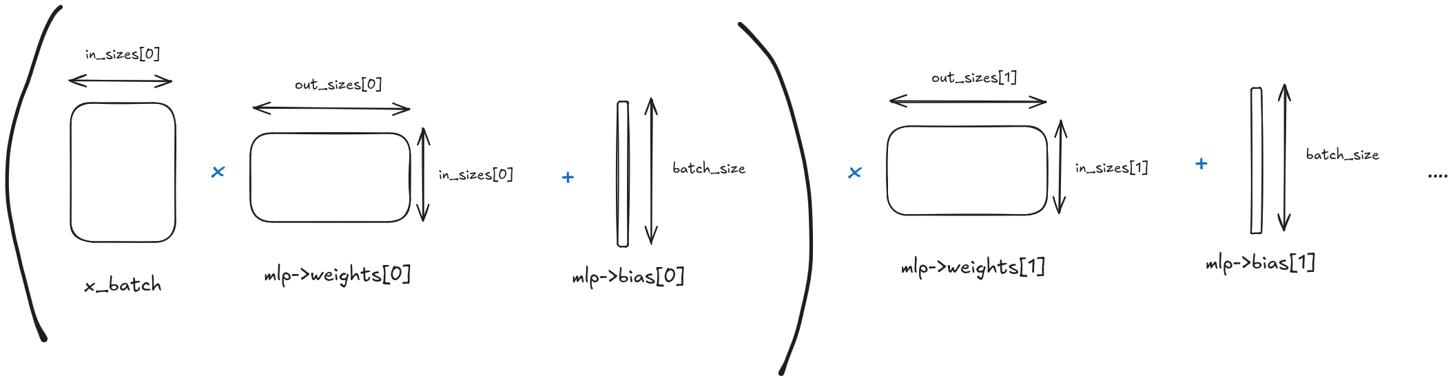
variable *forward_batch_multilayer_perceptron(multilayer_perceptron *mlp,
                                              variable *x_batch) {
  variable *output = x_batch;
  for (int i = 0; i < mlp->n_layers; i++) {
    output = matmul_variable(output, mlp->weights[i]);
    output = add_variable(output, mlp->bias[i]);
    switch (mlp->activations[i]) {
    case LINEAR:
      break;
    case RELU:
      output = relu_variable(output);
      break;
    case SIGMOID:
      output = sigmoid_variable(output);
      break;
    case SOFTMAX:
      output = softmax_variable(output, 1);
      break;
    case TANH:
      output = tanh_variable(output);
      break;
    default:
      break;
    }
  }

  return output;
}

The backward pass

For the training phase we need to define a loss function that we apply at the last layers output and then propagate the gradients backward through the network using the backward pass. This involves computing the gradients of the loss with respect to each weight and bias in the network and then updating these parameters using a gradient-based optimization method, such as stochastic gradient descent (SGD). The backward pass ensures that the network parameters are adjusted in a direction that minimizes the loss, thereby improving the model’s performance over successive epochs and batches.

void train_multilayer_perceptron(multilayer_perceptron *mlp,
                                 variable **x_batches, variable **y_batches,
                                 int n_batches, int n_epochs,
                                 NDARRAY_TYPE learning_rate,
                                 variable *(*loss_fn)(variable *, variable *)) {

  variable **weights = (variable **)malloc(mlp->n_layers * sizeof(variable *));
  variable **bias = (variable **)malloc(mlp->n_layers * sizeof(variable *));
  for (int i = 0; i < n_epochs; i++) {
    for (int j = 0; j < n_batches; j++) {
      variable *x_batch = shallow_copy_variable(x_batches[j]);
      variable *y_batch = shallow_copy_variable(y_batches[j]);
      variable *y_hat_batch = forward_batch_multilayer_perceptron(mlp, x_batch);
      variable *loss_batch = loss_fn(y_hat_batch, y_batch);

      zero_grad_multilayer_perceptron(mlp);
      backward_variable(loss_batch);
      if (j % 100 == 0) {
        printf("Epoch %d, batch %d, loss: %f\n", i, j,
               sum_all_ndarray(loss_batch->val));
      }
      update_multilayer_perceptron(mlp, learning_rate);

      for (int k = 0; k < mlp->n_layers; k++) {
        weights[k] = shallow_copy_variable(mlp->weights[k]);
        bias[k] = shallow_copy_variable(mlp->bias[k]);
      }

      free_graph_variable(&loss_batch);

      for (int k = 0; k < mlp->n_layers; k++) {
        mlp->weights[k] = weights[k];
        mlp->bias[k] = bias[k];
      }
    }
  }
  free(weights);
  free(bias);
}

The update_multilayer_perceptron function adjusts the weights and biases of each layer in the multilayer perceptron using the gradients computed during the backward pass. For each layer, it scales the gradients of the weights and biases by the learning rate.

void update_multilayer_perceptron(multilayer_perceptron *mlp,
                                  NDARRAY_TYPE learning_rate) {
  ndarray *place_holder;
  ndarray *temp;
  for (int i = 0; i < mlp->n_layers; i++) {
    place_holder = mlp->weights[i]->val;
    temp = multiply_ndarray_scalar(mlp->weights[i]->grad, learning_rate);
    mlp->weights[i]->val = subtract_ndarray_ndarray(mlp->weights[i]->val, temp);
    free_ndarray(&place_holder);
    free_ndarray(&temp);

    place_holder = mlp->bias[i]->val;
    temp = multiply_ndarray_scalar(mlp->bias[i]->grad, learning_rate);
    mlp->bias[i]->val = subtract_ndarray_ndarray(mlp->bias[i]->val, temp);

    free_ndarray(&place_holder);
    free_ndarray(&temp);
  }
}

For more info check multilayer_perceptron.c

Tests

ndarray, variable and multilayer_perceptron structures were tested by comparing the outputs of each function against their counterparts in popular libraries like NumPy and PyTorch, using the libmocka-c framework for unit testing.

For instance, consider the test for the sigmoid operation:

This Python function generates test data for unary operations like the sigmoid function. It creates random input data x, computes the output y using the specified unary operation, and performs a backward pass with a random gradient z. The input, output, and gradients are saved to files for comparison.

def generate_unary_op_test_data(test, output_dir, unary_op, x_shape):
    dir_path = os.path.join(output_dir, test)
    if not os.path.exists(dir_path):
        os.makedirs(dir_path)
    x = torch.rand(x_shape, dtype=torch.double, requires_grad=True)
    y = unary_op(x)
    z = torch.rand(x_shape, dtype=torch.double, requires_grad=True)
    y.backward(z)
    save_ndarray_to_file(os.path.join(dir_path, "x.txt"), x.detach().numpy())
    save_ndarray_to_file(os.path.join(dir_path, "y.txt"), y.detach().numpy())
    save_ndarray_to_file(os.path.join(dir_path, "z.txt"), z.detach().numpy())
    save_ndarray_to_file(os.path.join(dir_path, "x_grad.txt"), x.grad.detach().numpy())

# test_sigmoid_variable
    n = 10
    x_shape = (n, n)
    generate_unary_op_test_data(
        "test_sigmoid_variable", args.output_dir, torch.sigmoid, x_shape
    )

In the corresponding C test:

static void test_sigmoid_variable(void **state) {
  (void)state;
  char path[256];

  snprintf(path, sizeof(path), "%s/test_sigmoid_variable/x.txt", dataDir);
  ndarray *x = read_ndarray(path);

  snprintf(path, sizeof(path), "%s/test_sigmoid_variable/y.txt", dataDir);
  ndarray *y = read_ndarray(path);

  snprintf(path, sizeof(path), "%s/test_sigmoid_variable/z.txt", dataDir);
  ndarray *z = read_ndarray(path);

  snprintf(path, sizeof(path), "%s/test_sigmoid_variable/x_grad.txt", dataDir);
  ndarray *x_grad = read_ndarray(path);

  variable *var_x = new_variable(x);
  variable *var_y_hat = sigmoid_variable(var_x);
  free_ndarray(&(var_y_hat->grad));
  var_y_hat->grad = z;
  backward_variable(var_y_hat);

  assert_true(is_equal_ndarray(var_y_hat->val, y, NDARRAY_TYPE_EPSILON));
  assert_true(is_equal_ndarray(var_x->grad, x_grad, NDARRAY_TYPE_EPSILON));

  free_ndarray(&x);
  free_ndarray(&y);
  free_ndarray(&x_grad);

  free_graph_variable(&var_y_hat);
}

This C function reads the previously generated test data, performs the sigmoid operation on the ndarray encapsulated in a variable, and runs the backward pass. It then compares the resulting values and gradients to the expected outputs using assertions to ensure they are within a specified tolerance (NDARRAY_TYPE_EPSILON). This approach guarantees that the C implementation behaves correctly and consistently with the reference implementations in NumPy and PyTorch.

These unit tests were done for all the function, for more info check here

Examples

MNSIT

The MNIST dataset, consisting of 70,000 handwritten-digit images, is a classic benchmark for machine learning algorithms. It involves classifying digits from 0 to 9, providing an excellent test for our multilayer perceptron implementation. The following example demonstrates the setup, training, and evaluation of the model on the MNIST dataset.

Our model will be a 4 layer neural network with the following dimensions and activation function:

int n_layers = 4;
int in_sizes[] = {28 * 28, 64, 32, 16};
int out_sizes[] = {64, 32, 16, 10};
activation_function activations[] = {SIGMOID, SIGMOID, SIGMOID, LINEAR};

We will train our model with the following parameters:

int batch_size = 64;
int n_epochs = 100;
NDARRAY_TYPE learning_rate = 0.01;

and since this is a classification problem we need to define the loss function which is the cross entropy loss

variable *cross_entropy_loss(variable *logits, variable *y) {
  variable *y_hat_exp = exp_variable(logits);
  variable *y_hat_sum = sum_variable(y_hat_exp, 1);
  ndarray *temp = full_ndarray(y_hat_sum->val->dim, y_hat_sum->val->shape,
                               NDARRAY_TYPE_EPSILON);
  variable *y_hat_log_sum =
      log_variable(add_variable(y_hat_sum, new_variable(temp)));
  free_ndarray(&temp);

  variable *y_hat_softmax = subtract_variable(logits, y_hat_log_sum);

  variable *product = multiply_variable(y, y_hat_softmax);
  variable *neg_product = negate_variable(product);
  variable *loss = sum_variable(neg_product, 1);

  free_ndarray(&(loss->grad));
  loss->grad = ones_ndarray(loss->val->dim, loss->val->shape);
  return loss;
}

If we start the training we can see that indeed our model is learning:

Epoch 0, batch 0, loss: 153.069234
Epoch 0, batch 100, loss: 149.035196
Epoch 0, batch 200, loss: 146.707832
Epoch 0, batch 300, loss: 118.086699
Epoch 0, batch 400, loss: 86.300584
Epoch 0, batch 500, loss: 66.593495
Epoch 0, batch 600, loss: 59.607119
Epoch 1, batch 0, loss: 57.373467
Epoch 1, batch 100, loss: 53.599278
Epoch 1, batch 200, loss: 33.338024
Epoch 1, batch 300, loss: 29.048711
Epoch 1, batch 400, loss: 38.811830
Epoch 1, batch 500, loss: 24.286488
Epoch 1, batch 600, loss: 22.726048
Epoch 2, batch 0, loss: 28.801350
Epoch 2, batch 100, loss: 35.327724
Epoch 2, batch 200, loss: 14.522009
Epoch 2, batch 300, loss: 14.909454
Epoch 2, batch 400, loss: 17.792573
Epoch 2, batch 500, loss: 6.376877
Epoch 2, batch 600, loss: 13.702117
Epoch 3, batch 0, loss: 19.182989
Epoch 3, batch 100, loss: 28.739773
Epoch 3, batch 200, loss: 11.350802
Epoch 3, batch 300, loss: 13.056788
Epoch 3, batch 400, loss: 11.537156
Epoch 3, batch 500, loss: 4.421002
Epoch 3, batch 600, loss: 10.465591
Epoch 4, batch 0, loss: 15.420338
Epoch 4, batch 100, loss: 23.214068
Epoch 4, batch 200, loss: 10.336427
Epoch 4, batch 300, loss: 10.720565
Epoch 4, batch 400, loss: 8.834916
Epoch 4, batch 500, loss: 3.295116

You can check the full example here

Paint

This is more of a fun example, where we only use the forward pass to create a sort of neural network shader, i.e., we input a vector that represents the coordinates of a pixel in the image, and we get back a vector that represents the color.

I landed on the following model:

int layer_size = 32;
multilayer_perceptron *mlp = new_multilayer_perceptron(
      9, batch_size,
      (int[]){3, layer_size, layer_size, layer_size, layer_size, layer_size,
              layer_size, layer_size, layer_size},
      (int[]){layer_size, layer_size, layer_size, layer_size, layer_size,
              layer_size, layer_size, layer_size, 3},
      (activation_function[]){TANH, TANH, TANH, TANH, TANH, TANH, TANH, TANH,
                              SIGMOID},
      (random_initialisation[]){NORMAL, NORMAL, NORMAL, NORMAL, NORMAL, NORMAL,
                                NORMAL, NORMAL, NORMAL});

Using the following coordinates as an input:

ndarray *x = zeros_ndarray(2, (int[]){height * width, 3});
for (int i = 0; i < height; i++) {
  for (int j = 0; j < width; j++) {
    x->data[3 * (i * width + j)] = ((NDARRAY_TYPE)i / height - 0.5) * zoom;
    x->data[3 * (i * width + j) + 1] = ((NDARRAY_TYPE)j / width - 0.5) * zoom;
    x->data[3 * (i * width + j) + 2] =
        sqrt(pow((NDARRAY_TYPE)i / height - 0.5, 2.0) +
             pow((NDARRAY_TYPE)j / width - 0.5, 2.0)) *
        zoom;
  }
}

Here is an example of what you can get:

You can check the full example here

Conclusion

This Autograd library in C demonstrates essential neural network operations and automatic differentiation through a simplified, custom implementation. The code includes key components like tensor operations, neural network layers, and forward and backward propagation, all aimed at providing a clear educational example. Note that this implementation is primarily for instructional purposes, as real-world libraries are more complex and optimized for performance.